Reuven Glick Responds! The Currency Unions and Trade Debate Rages On...

Previously, I reviewed the Currency Unions and Trade Literature here, and then shared some of my students' referee reports of a recent Glick and Rose (2016) paper here. My undergraduates were quite skeptical.

In fact, I first wrote a paper on currency unions and trade as my class paper when I was a grad student in Alan Taylor's excellent course in Open-Economy Macro/History. A doubling of trade due to a currency union looked like a classic case of "endogeneity" to me. Currency Unions are like marriages, they don't form or break apart for no reason. They are as non-random a treatment as you'll find. In addition, we know from Klein and Shambaugh's excellent work that direct pegs seem to have a much smaller impact on trade, and that indirect pegs -- which probably are formed randomly -- have no effect at all. Thus we know that the effect of currency unions doesn't operate via exchange rate volatility, the most plausible channel. Also, the magnitude of the effects bandied about are much too large to be believed. Consider that Doug Irwin finds that the Smoot-Hawley tariff reduced trade by 4-8%.  How plausible is it that currency unions have an impact at least 12 times larger? Or the Euro six times larger? It isn't. A 5% increase in trade still implies an increase of tens of billions of dollars for the EU -- probably still too large. My intuition is that something on the order of .05-.5% would be plausible, but too small to estimate.

Since I was skeptical, I fired up Stata. It then took me approximately 30 minutes to make the magical -- yes, magical -- effect of currency unions on trade disappear, at least for one major sub-sample -- former UK colonies. It took only a bit more time to notice that the results were also driven by wars and missing data, but it was still a quick paper.

In any case, to his credit, Reuven Glick responds, making many thoughtful points. Here he is:

My co-author, Andy Rose, already responded to the comments on your blogsite about our recent EER paper. I'd like to offer my additional one-shot responses to your comments of March 24, 2017 and your follow-up on April 24, 2017.

•As Andy noted, we find significant effects for many individual currency unions (CUs), not just for those involving the British pound and former UK colonies. Yes, the magnitude of the trade effects varies across these unions, but that’s not surprising. So the “magical” currency union effect doesn’t disappear, even when attributing the UK-related effects to something other than the dissolution of pound unions. 

There is a pattern in this literature. You guys find a large trade impact result, and then somebody points out that it isn't robust -- in short, that the effect does disappear. For example, Bomberger (no paper on-line; but Rose helpfully posted his referee report here) showed that your earlier results go away for the colonial sample with the inclusion of colony-specific time trends, while Berger and Nitsch have already showed that a simple time trend kills the Euro impact on trade. Each time you guys then come back with a larger data set, and show that the impact is robust. However, the lessons from the literature curiously do not get internalized; the controls which reversed your previous results forgotten.

Since you mention the UK, let's have a look at a simple plot of trade between the UK and its former colonies vs. the UK and countries which it had currency unions. What you see below are the dummies plotted in a gravity regression for the UK with its former colonies vs. countries that ever had a UK currency union. Note that the UK had something like 60+ colonies while there are only 20-something countries which had currency unions, only one of them a non-colony. What it shows is that the evolution of trade between the UK and its former colonies is quite similar to the evolution of trade between the UK and countries which shared a CU with. The blue bars (axis at left), then show the dates of UK currency union dissolutions, mostly during the Sterling Crisis of the 1960s. What one sees is that there was a gradual decaying of trade for both UK colonies and countries ever in a currency union.

So, yes, including a time trend control does in fact make the "magical" result go away. In my earlier paper, I got an impact of 108% for UK Currency Unions with no time trend control, but -3.8% (not statistically significant) when I include a simple UK colony*year trend control. That's a fairly stark difference from the introduction of a mild control. And, in your earlier paper (Glick and Rose, 2002), the UK colonial sample comprises one-fifth of the CU changes with time series variation in the data. In addition, the disappearance of the CU effect for UK CUs raises the question of how robust it is for other subsamples, where CU switches are also not exogenous -- think India-Pakistan. It turns out that almost none of it is robust. Yet, you do nothing to control for the impact of decolonization in your most recent work, nor do you ask what might be driving your results in other settings.

The thing is, it isn't just that you didn't see my paper (which I emailed to you). Your coauthor clearly refereed Bomberger's paper, which looks to me like a case of academic gatekeeping. I love academia, damnit! Bomberger deserved better than what he got. I want the profession to produce results people can believe in. With all due respect, you guys are repeat offenders at this stage.  If this was your first offense, I would not have been so aggressive. And yes, I'll confess to having been put off by the fact that you thanked me, even though I did not comment on the substance of your paper, but did not cite me.


•We tried to control for as many things as possible by including the usual variables, such as former colonial status, as well as appropriate fixed effects, such as country-year and pair effects. Yes, one can always think of something that was left out. For example, if you’re concerned about the effects of wars and conflicts, check out my paper with Alan Taylor (“Collateral Damage: Trade Disruption And The Economic Impact Of War,” RESTAT 2010), where we find that that currency unions still had sizable trade effects, even after controlling for wars (see Table 2). Granted the data set only goes up to 1997 in that paper, and we don’t address the effects of the end of the Cold War, the dissolution of the USSR, and the Balkan wars. That might make an interesting project for one of your graduate students to pursue.

OK, sure. I would like to believe that figuring out what was driving the CU effect on trade was incredibly difficult to figure out, and that I was able to solve the puzzle only via genius, but the reality is that others (such as Bomberger; others also mentioned decolonization as a factor too, or reversed earlier versions of the CU effect, and let's not forget my undergraduates), also had prescient critiques. I don't get the sense that you guys really searched very hard for alternative explanations (India and Pakistan hate each other!) for the enormous impacts you were getting. It looks to me more like you included standard gravity controls and then weren't overly curious about what was driving your results. As my earlier paper notes, it's actually quite difficult to find individual examples of currency unions in which trade fell/increased only right after dissolution/formation, without having a rather obvious third factor driving the results (decolonization, communist takeover, the EU). Even in your recent paper, you find strong "pre-treatment trends" -- that trade is declining long before a CU dissolution. In modern Applied Micro, the existence of strong pre-treatment trends is more evidence that the treatment is not random. It should have been a red flag.


•I agree that it is important to disentangle the effects of EMU from those of other forms of European trade integration, such as EU membership. In our EER paper we included an aggregated measure that captures the average effect of all regional trade agreements (RTAs). Of course, aggregating all such arrangements together does not allow for possible heterogeneity across different RTAs. To see if this matters, see a recent paper of mine (“Currency Unions and Regional Trade Agreements: EMU and EU Effects on Trade,” Comparative Economic Studies, 2017) where I separate out the effects of EU and other RTAs so as to explicitly analyze how membership in EU affects the trade effects of EMU. I also look at whether there are differences in the effects between the older and newer members of the EU and EMU, something that should be of interest to your students interested in East European transition economies. I find that the EMU and EU each significantly boosted exports, and allowing separate EU effects doesn't "kill" the EMU effect. Most importantly, even after controlling for the EU effects, EMU expanded European trade by 40% for the original members. The newer members have experienced even higher trade as a result of joining the EU, but more time and a longer data set is necessary to see the effects of their joining EMU. 


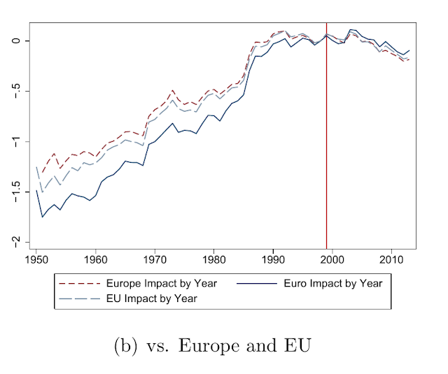
OK, but a 40% increase that you find in your 2017 paper is already 25% smaller than the 50% you guys argue for in your 2016 paper. At a minimum, the result seems sensitive to specification. I'm not convinced that a single 0/1 RTA dummy for all free trade agreements is remotely enough to control for the entire history of European integration, from the Coal & Steel Community, to the ERM and EU. Also, 0/1 dummies imply that the impact happens fully by year 1, and ignores dynamics -- part of my earlier critique. If two countries go from autarky to free trade, the adjustment should take more than just one year.  On a quick look at your 2017 paper, I'd say: I'd like to see you control for an Ever EU*year interactive fixed effect. If you do that, you'll kill the EMU dummy much like the EMU did to the Greek economy. I'd also like to see you plot the treatment effects over time, as I did in my previous post. (Here it is again:)

Once again, I don't know how you can look at this above and cling to a 40 or 50% impact of the EMU. The pre-EMU increase in trade mostly happens by 1992. This increase happens for all EU countries, and indeed all Western European countries. Those that eventually joined the Euro even have trade increasing faster than EU or all Western European countries even before the EMU. If you ignore this pre-trend, you could get an impact of several percent at most for the difference between the Euro vs. EU/Europe in the graph above by 2013, but that difference won't be statistically significant.


•Andy and I agree that the endogeneity of CUs could be a concern, and suggested that employing matching estimation might be one way to approach the issue. Perhaps this would be another good assignment for one of your graduate students, who are interested in doing more than “seek and destroy.”

I agree with this. The point shouldn't be to destroy, but to provide the best estimate possible. I would be more than happy to join forces with you guys and one of my graduate students in writing a proper mea culpa, to nip this literature in the bud. It certainly would take a lot of intellectual integrity to do this, and you should be commended for it if you would like to do this. (Although, I'd note that this your results have already been reversed.) Your new paper has a larger data set, but is sensitive to the same concerns already extant in the literature.

•Lastly, our recent EER paper has over 40 references; sorry we didn’t include you. Please note that your citation date for our paper should be corrected; the paper was published in 2016, not 2017.

OK. You also should have added in a citation for Bomberger's unpublished manuscript, who killed your results on a key subsample.

One question -- now that you guys have my earlier paper in hand, and know that a time trend kills the UK CU effect, for example, and know that missing data and wars are driving the other result, and now that you've seen my figure above showing that the EMU increased trade by at most a couple percent, do you still believe that currency unions double trade, on average? Or, which part of my earlier paper did you not find convincing? And which parts were convincing?

Read More

How Bad is Peer Review? Evidence From Undergraduate Referee Reports on the Currency Unions and Trade Lit

In a recent paper, Glick and Rose (2016) suggest that the Euro led to a staggering 50% increase in trade. To me, this sounded a bit dubious, particularly given my own participation in the previous currency unions and trade literature (which I wrote up here; my own research on this subject is here). This literature includes papers by Robert Barro that imply that currency unions increase trade on a magical 10 fold basis, and a QJE paper which suggests that currency unions even increase growth. In my own eyes, the Euro has been a significant source of economic weakness for many European countries in need of more stimulative policies. (Aside from the difficulty of choosing one monetary policy for all, it also appears that MP has been too tight even for some of the titans of Northern Europe, including Germany. But that's a separate issue...)

Given my skepticism, I gave my sharp undergraduates at NES a seek-and-destroy mission on the Euro Effect on trade. Indeed, my students found that the apparent large impact of the Euro, and other currency unions, on trade is in fact sensitive to controls for trends, and is likely driven by omitted variables. One pointed out that the Glick and Rose estimation strategy implicitly assumes that the end of the cold war had no impact on trade between the East and the West. Several of the Euro countries today, such as the former East Germany, were previously part of the Warsaw Pact. Any increase in trade between Eastern and Western European countries following the end of the cold war would clearly bias the Glick and Rose (2016) results, which naively compare the entire pre-1999 trade history with trade after the introduction of the Euro.  Indeed, Glick and Rose assume that the long history of European integration (including the Exchange Rate Mechanism) culminating with the EU had no effect on trade, but that switching to the Euro from merely fixed exchange rates resulted in a magical 50% increase. Several of my undergraduates pointed out that this effect goes away by adding in a simple time trend control. Others noted that the authors only clustered in one direction, rather than in two or three directions one might naturally expect. In some cases, multi-way clustering reduced the t-scores substantially, although didn't seem to be critical. One student reasoned that the preferred regression results from GR (2016) don't really suggest that CUs have a reliable impact on trade. The estimates from different CU episodes are wildly different --  GR found that some CUs contract trade by 80%, while others have no statistically significant effect, some have a large effect, while others have an effect that is simply too large to be believed (50-140%). Many of my students noted that there is an obvious endogeneity problem at play -- countries don't decide to join or leave currency unions randomly -- and the authors did nothing to alleviate this concern. The currency union breakup between India and Pakistan is but one good example of the non-random nature of CU exits.

You'd think that a Ph.D.-holding referee for an academic journal which is still ranked in the Top 50 (Recursive, Discounted, last 10 years) might at least be able to highlight some of these legitimate issues raised by undergraduates. You might imagine that a paper which makes some of the errors above might not get published, especially if, indeed, star economists face bias in the publication system. You might also imagine that senior economists, tenured at Berkeley/at the Fed, might not make these kinds of mistakes which can be flagged by undergraduates (no matter how bright) in the first place. You'd of course be wrong.

The results reported and the assumptions used to get there are so bad that you get the feeling these guys could have gotten away with writing "Get me off your fucking mailing list" a hundred times to fill up space.

Before ending I should note that I do support peer review, and also believe that economics research is incredibly useful when done well. But science is also difficult. This example merely highlights that academic economics still has plenty of room for improvement, and that a surprisingly large fraction of published research is probably wrong. I should also add that I don't mean to pick on this particular journal -- if a big name writes a bad article, it is only a question of which journal will accept it. However, this view of the world suggests that comment papers, replications, and robustness checks deserve to be more valued in the profession than they are at present. Much of the problem with that line of work also stems from almost a willful ignorance of history. Thus, it's also sad to see departments such as MIT scale back their economic history requirements in favor of more math. I don't see this pattern resulting in better outcomes.


Update: Andrew Rose responds in the comments. Good for him! Here I consider each of his points.

Rose wrote: "-Get them to explain how that they could add a time trend to regression (2), which is literally perfectly collinear with the time-varying exporter and importer fixed effects."

Sorry, but a Euro*year interactive trend, or, indeed, any country-pair trend, is not going to even close to co-linear with time-varying importer and exporter year fixed effects. The latter would be controlling for a general country trend, but not for trends in country-pair specific relationships. To be fair, regression of one trending variable on another with no control for trends is the most common empirical mistake people make when running panel regressions.

-Explain to them how time-varying exporter/importer fixed effects automatically wipe out all phenomena such as the effects of the cold war and the long history of European monetary integration.

Sorry, but that's also not the case. A France year dummy, to be concrete, won't do it. That would pick up trade between France and all other countries, including EU, EMU, and former Warsaw Pact countries. You'd need to put in a France*EU interactive dummy, for example. But such a dummy will kill the EMU. Below, I plot the evolution of trade flows over time (dummies in the gravity equation) for (a) all of Western Europe, (b) Western European EU countries, and (c) the original entrants to the Euro Area (plus Greece). What you can see is that, while trade between EMU countries was much higher after the Euro than before (your method), most of the increase happened by the early 1990s, in fact. Relative to 1998, trade even declined a bit by 2013. There's nothing here to justify pushing a 50% increase.

Rose also indicated that my undergraduates should "Read the paper a little more carefully. For instance, consider; and a) the language in the paper about endogeneity b) Table 7 which explicitly makes the point about different currency unions. "


Actually, let's do that. When I search for "endogeneity" in the article, the first hit I get is on page 8, where it is asserted that including country-pair fixed effects controls for endogeneity. Indeed, it does control for time-invariant endogeneity. But if countries, such as India and Pakistan, have changing relations over time (such as before and after partition), this won't help.

The second hit I get is footnote 7: "Our fixed‐effects standard errors are also robust. We do not claim that currency unions are formed exogenously, nor do we attempt to find instrumental variables to handle any potential endogeneity problem. For the same reason we do not consider matching estimation further, particularly given the sui generis nature of EMU." [the bold is mine.]

Actually, a correction here: my undergrads reported that the FE standard errors are actually clustered, but this is a minor point. You may not claim that currency unions are formed exogenously, but, as you admit, your regression results do nothing to try to reduce the endogeneity problem. And, this, despite the fact that I had already shared my own research with you (ungated version), which showed that your previous results were sensitive to omitting CU switches coterminous with Wars, ethnic cleansing episodes, and communist takeovers.

Also, the "For the same reason" above is a bit strange. The sentence preceeding it doesn't give a reason why you don't try to handle the endogeneity problem. The reason is? In fact, a matching-type estimator would be advisable here.

Lastly, in your discussion of Table 7, I see you note that it implies widely varying treatment effects of CUs on trade. But I like my undergraduates interpretation of this as casting doubt on the exercise. Many of the individual results, including an 80% contraction for some currency unions, are simply not remotely plausible. The widely varying results are almost certainly due to wildly different endogeneity factors affecting each group of currency unions, not due to wildly different treatment effects.

Update 2: Reuven Glick points out that their paper was published in 2016, not 2017. I've fixed this above.

Read More

AFL experiments, or please eat your brötli

When messing around with AFL, you sometimes stumble upon something unexpected or amusing. Say,
having the fuzzer spontaneously synthesize JPEG files,
come up with non-trivial XML syntax,
or discover SQL semantics.

It is also fun to challenge yourself to employ fuzzers in non-conventional ways. Two canonical examples are having your fuzzing target call abort() whenever two libraries that are supposed to implement the same algorithm produce different outputs when given identical input data; or when a library produces different outputs when asked to encode or decode the same data several times in a row.

Such tricks may sound fanciful, but they actually find interesting bugs. In one case, AFL-based equivalence fuzzing revealed a
bunch of fairly rudimentary flaws in common bignum libraries,
with some theoretical implications for crypto apps. Another time, output stability checks revealed long-lived issues in
IJG jpeg and other widely-used image processing libraries, leaking
data across web origins.

In one of my recent experiments, I decided to fuzz
brotli, an innovative compression library used in Chrome. But since it's been
already fuzzed for many CPU-years, I wanted to do it with a twist:
stress-test the compression routines, rather than the usually targeted decompression side. The latter is a far more fruitful
target for security research, because decompression normally involves dealing with well-formed inputs, whereas compression code is meant to
accept arbitrary data and not think about it too hard. That said, the low likelihood of flaws also means that the compression bits are a relatively unexplored surface that may be worth
poking with a stick every now and then.

In this case, the library held up admirably - spare for a handful of computationally intensive plaintext inputs
(that are now easy to spot due to the recent improvements to AFL).
But the output corpus synthesized by AFL, after being seeded just with a single file containing just "0", featured quite a few peculiar finds:

• 
  

  
  Strings that looked like viable bits of HTML or XML:
  <META HTTP-AAA IDEAAAA,
  DATA="IIA DATA="IIA DATA="IIADATA="IIA,
  </TD>.
  

  
  
  
• 
  

  
  Non-trivial numerical constants:
  1000,1000,0000000e+000000,
  0,000 0,000 0,0000 0x600,
  0000,$000: 0000,$000:00000000000000.
  

  
  
  
• 
  

  
  Nonsensical but undeniably English sentences:
  them with them m with them with themselves,
  in the fix the in the pin th in the tin,
  amassize the the in the in the inhe@massive in,
  he the themes where there the where there,
  size at size at the tie.
  
  

  
  
  
• 
  

  
  Bogus but semi-legible URLs:
  CcCdc.com/.com/m/ /00.com/.com/m/ /00(0(000000CcCdc.com/.com/.com
  

  
  
  

• 
  

  
  Snippets of Lisp code:
  )))))))))))))))))))))))))))))))))))))))))))))))))))))))))))))))))))))))))))))))))))))))).
  

  
  
  

The results are quite unexpected, given that they are just a product of randomly mutating a single-byte input file and observing the code coverage in a simple compression tool. The explanation is that brotli, in addition to more familiar binary coding methods, uses a static dictionary constructed by analyzing common types of web content. Somehow, by observing the behavior of the program, AFL was able to incrementally reconstruct quite a few of these hardcoded keywords - and then put them together in various semi-interesting ways. Not bad.

Read More

The St. Louis Fed's Macroeconomic Outlook

St. Louis Fed president James Bullard recently gave this speech on the U.S. macroeconomic outlook. The key themes of his talk were:

1. The U.S. economy has converged to a low-growth, low-safe-real-interest-rate regime, a situation that is unlikely to change dramatically over the near future;
2. The Fed can afford to take a wait-and-see posture in regard to possible changes in U.S. fiscal and regulatory policies;
3. The U.S. policy rate can remain relatively low for now and that doing so is consistent with the dual mandate;
4. Now may be a good time for the FOMC to consider allowing the balance sheet to shrink in nominal terms.

What does Bullard have in mind when he speaks of a low-growth "regime?" The usual way of interpreting development dynamics is that long-run growth is more or less stable and that deviations from this stable trend represent "cyclical" mean-reverting departures from trend. And if it's "cyclical," then it's temporary--we should be forecasting reversion to the mean in the near future--like the red forecasting lines in the picture below.

This view of the world can lead to a series of embarrassing forecast errors. Since the end of the Great Recession, for example, you would have forecast several recoveries, none of which have materialized.

But what if that's not the way growth happens? Suppose instead that growth occurs in decade-long spurts? Something like this.

This view of the development process does not say we're presently stuck forever in a low-growth regime. It simply suggests that we have no idea when the economy will once again embark on a higher (or heaven-forbid, lower) growth regime and that in the meantime our best forecast is for continued low-growth for the foreseeable future.

A reader suggests plotting the annualized ten-year growth rate quarter-by-quarter. Here is what it looks like:

What determines a growth regime? Government policies may play a role. Or perhaps it's just the way economies grow. There is no God-given rule which says that productivity growth must at all times proceed in a straight line. Here is the San Francisco Fed's measure of total factor productivity:

Note that the most recent productivity growth slowdown occurred well before the financial crisis.

The notion that the economy has converged to a low-growth regime is also evident in a variety of labor market measures. The prime-age unemployment rate is essentially back to its recent historical average, for example.

Measures of prime-age employment and participation still have a way to go, but arguably not very much.

Next, what does he have in mind when he speaks of a "low-safe-real-interest-rate regime?" Bullard associates the "safe-real-interest-rate" with the expected real rate of return on (nominally) safe U.S. treasury debt (which he labels "r-dagger"). Operationally, he uses the one-year U.S. treasury yield minus a measure of year-over-year inflation (e.g., the Dallas trimmed-mean inflation). Below I plot "r-dagger" using year-over-year PCE inflation. I also plot an hypothetical "r-star" interest rate which (as suggested by theory) should track the expected growth rate of real per capita consumption expenditure.

The (theoretical) real interest rate (as measured here by consumption growth)--the blue line--is on average high in high-growth regimes and low in low-growth regimes (the 1950s provide an exception). The r-dagger interest rate appears to move broadly with r-star (the early 1980s provide a dramatic exception).  The gap between r-star and r-dagger could be interpreted as a risk-premium (or a liquidity premium). The secular decline in r-dagger since the early 1980s reflects a number of factors. Inflation expectations fell and became anchored under Volcker. And since at least 2000, there's been an ever-expanding global demand for safe assets which are used extensively as collateral in shadow banking, as safe stores of wealth in emerging economies, and as objects that fulfill growing regulatory requirements (Dodd-Frank and Basel III). Evidently, Bullard does not believe that the appetite for these safe assets is likely to dissipate any time soon.

 

As for inflation, headline PCE inflation has only recently ticked back up close to the Fed's official 2% target. Nominal wage growth has also ticked up recently, but remains rather muted. The growth in real wages remains low--which is consistent with the U.S. economy operating in a low-growth regime.

Market-based measures of long-run inflation expectations appear well-anchored. Below I plot the 10-year breakeven inflation rate (expected inflation 10 years out) and the real yield on the 10-year U.S. treasury (blue line).

Given these observations, what's the rush to raise the policy rate?

At the same time, Bullard is suggesting that it might be a good time to think about reducing the size of the Fed's balance sheet. He notes that recent FOMC policy is putting upward pressure at the short end of the yield curve (via recent policy rate increases) at the same time putting downward pressure at the long end of the yield curve (via the long-term securities purchased in the LSAP). Bullard notes that "this type of twist operation does not appear to have theoretical basis." In fact, it's not clear what policy should aim for (if anything at all) in terms of influencing the slope of the yield curve.

Nevertheless, there are some good reasons to shrink the balance sheet (I provide a reason for keeping it large here). First, if there is indeed a shortage of safe assets, why is the Fed buying them up (replacing them with reserves that only depository institutions can access directly)? Ending the reinvestment program would release additional safe assets for the market, the effect of which would be to increase yields on safe assets (a good thing to the extent higher yields represent diminished liquidity premia.) Second, ending reinvestment (especially in MBS) would be a good move politically. One concern about ending reinvestment seems centered around the possibility of creating another "taper tantrum" event. But it seems unlikely that disruption in the bond market would occur if the policy change is communicated clearly and with plenty of advance notice.

Read More

How to integrate querydsl in your javaee7 project

This guide requires knowledge on:

• maven
• git
• eclipse
• querydsl
• wild fly

We will show you how to modify the javaee7-archetype project to integrate querydsl. For those who do not know, it is a library to unify queries in java. What I like more about it is that you can fluently construct your api. For more info refer to: http://www.querydsl.com/static/querydsl/4.1.3/reference/html_single/

Follow this guide to setup your project:
http://czetsuya-tech.blogspot.com/2017/04/how-to-setup-arquillian-testing-with.html
Take note, of the arquillian configuration, as we will need it later.

Since I am lazy :-), I will just provide the test project that I have created in GitHub: https://github.com/czetsuya/JavaEE7-QueryDSL-Demo

Things you should take notice:

• In resources I have added a JPAQueryFactoryProducer:
  

  @Produces
   public JPAQueryFactory produceJPQQueryFactory() {
    return new JPAQueryFactory(em);
   }
  

• Note that I have modified Member entity, added a BaseEntity and Identifiable interface.
• I have added a new package: com.broodcamp.javaee_querydsl_demo.repository and the classes inside it.
• I have also modified: MemberRegistrationTest, so that we can run the arquillian test correct.

To run arquillian simply execute this command inside your project in the terminal:

>mvn clean test -Parq-wildfly-managed

The test should run without error.

Read More

How to setup Arquillian testing with Wildfly

This tutorial requires:

• Knowledge with GIT
• Knowledge with archetype

Requirements:

• Wildfly
• eclipse

What to do:

1. In eclipse create a new maven project: File->New->Other, enter maven in the filter. Select Maven Project.
   
2. Click next, then next. In the filter enter "javaee". Select wildfly-javaee7-webapp-archetype.
   
3. Click next, enter group and artifact id.
4. Click finish. Your project should be created.
5. Open arquillian.xml in src/test/resources. Uncomment configuration section and set the jbossHome property:
   

   <?xml version="1.0" encoding="UTF-8"?>
   <arquillian xmlns="http://jboss.org/schema/arquillian"
    xmlns:xsi="http://www.w3.org/2001/XMLSchema-instance"
    xsi:schemaLocation="http://jboss.org/schema/arquillian
           http://jboss.org/schema/arquillian/arquillian_1_0.xsd">
   
    <!-- Force the use of the Servlet 3.0 protocol with all containers, as it 
     is the most mature -->
    <defaultProtocol type="Servlet 3.0" />
   
    <!-- Example configuration for a remote WildFly instance -->
    <container qualifier="wildfly" default="true">
     <!-- By default, arquillian will use the JBOSS_HOME environment variable. 
      Alternatively, the configuration below can be uncommented. -->
     <configuration>
      <property name="jbossHome">C:\java\jboss\wildfly-10.1.0.Final</property>
   <!--    <property name="javaVmArguments">-Xmx512m -XX:MaxPermSize=128m -->
   <!--                 -Xrunjdwp:transport=dt_socket,address=8787,server=y,suspend=y -->
   <!--             </property> -->
     </configuration>
    </container>
   
    <engine>
     <property name="deploymentExportPath">target/deployments</property>
    </engine>
   
   </arquillian>
   

6. Then in your terminal, go to your project directory and run:
   >mvn clean test -Parq-wildfly-managed
   >This run arquillian test using wildfly managed container.

It's actually a straightforward process. The tricky part is creating your test war. Open MemberRegistrationTest, to see what I mean. Sometimes it's useful to include an archive with all its dependencies than including one class at a time.

Read More

Sectoral and Occupational Trends in the U.S. Labor Market

The labor market is back to normal. Or so we are told. Here's the prime-age unemployment rate for the United States beginning in 1960.

Above we see the familiar cyclical asymmetry, in which the unemployment rate spikes up sharply at the onset of a recession and declines gradually during the recovery. As of today, the prime-age unemployment rate is at 4%, close to its recent historical norm. 

Other measures of labor market activity, however, tell a slightly different story. Here is the prime-age employment-to-population ratio. Employment took a big tumble during the recession--especially for males--and its taken a lot longer to recover than unemployment. In fact, we're not quite back to pre-recession average of about 80%. 

The reason employment has recovered more slowly than unemployment is because significant numbers of prime-age workers left the labor force in the aftermath of the Great Recession. This pattern has reversed only recently.

By these standard measures of aggregate labor market activity, the U.S. labor market appears close to "full employment." Nevertheless, there is still much anxiety concerning the present state and future course of the U.S. labor market. Much of this anxiety stems from the perennial concerns regarding the impact of international trade and technology on future employment opportunities. 

To assess the nature of these concerns, we have to move beyond the standard aggregate measures of labor market activity, which have remained relatively stable since 1990 in the face of growing trade deficits and technological progress. So if trade and technology are going to have an impact on employment opportunities, it's likely going to happen at the sectoral and/or occupational level. 

Of course, a changing allocation of human labor across sectors of the U.S. economy is nothing new. Here is the share of employment in agriculture and manufacturing since 1815. 

In 1815, 80% of employment was devoted toward the production of food. And for those of us who have never worked on a farm, here's how Charles H. Smith describes the venture in 1892:

“It’s about the meanest business I have ever experienced. It’s all fact—solemn fact – no romance, no poetry, no joke. It does seem to me that all this sort of work ought to be done by machinery or not to be done at all.” Source: Farm Life at the Turn of the Century.

As we can see, Smith got his wish. Over the centuries, machines have replaced most of human labor in the production of food. Was this a welcome development? Most of us today would likely answer in the affirmative. However, sectoral transformations like this also come at a cost, borne by those who are compelled to do the adjusting. A shovel that helps ease a manual burden is one thing. A combine harvester that renders a certain kind of labor redundant is another. When the demand for a certain type of labor in a given sector is diminished, what are workers to do? 

One thing they can do is employ their labor in the production of the machines that replaced their labor on the farm. And so youngsters left the family farm and immigrants flowed increasingly into the communities that offered employment in manufacturing and other sectors. I'm not sure how much of an improvement it was to substitute the drudgery of farm work with the drudgery of factory work, but it was probably an improvement in net terms (however small). The relatively high levels of comfort most Americans enjoy today did not come about until the latter half of the 20th century. And by that time, manufacturing employment (as a share of total employment) began its long secular decline. 

So, what accounts for the decline in manufacturing sector employment? According to Dean Baker, the U.S. trade deficit has a lot to do with it. 

Since 2000, employment in the U.S. manufacturing sector has dropped from about 17 million to 12 million workers. The sharp decline started with the "China shock" in 2001 (also a recession year). On the other hand, Germany has also experienced a decline in manufacturing sector employment while running trade surpluses. Arguably, the trade surpluses muted the secular decline in manufacturing employment in Germany, while the U.S. trade deficits exacerbated the process of structural readjustment. The trade deficit has almost surely had some impact on U.S. manufacturing employment, but it's hard for me to escape the conclusion that most of the sectoral reallocation of labor has been driven by technology. The next diagram tells the story. 

But it hardly matters to an individual worker whether they are displaced by a foreigner or an automaton. Where are the new jobs to be found and what are they paying? Are all of our good, high-paying manufacturing jobs being replaced by lousy low-paying service sector jobs? There is an element of truth to this. As Daniel Alpert points out, since the cyclical peak in 2007, the U.S. economy has added close to 7 million jobs. About 60% of these jobs appeared in the "low-wage, low-hours" sectors that account for about 36% of all private sector jobs; see table below. 

The picture is not quite as bleak as Alpert paints it. Andrew Spewak (my trusty RA) took it upon himself to produce this table. 

What this decomposition shows is that there is in fact substantial net job creation in high-wage/high-hour jobs in the service sector. The bleakness is heavily concentrated in manufacturing (which we know is in secular decline) and in construction (which is not in secular decline, but which hit a peak just prior to the housing crisis). 

Let's dig a little deeper and explore the task-based view of the labor market developed by Daron Acemoglu and David Autor (see here). According to this view, goods and services are produced by a set of tasks that can be performed by various inputs, like capital and labor. Tasks differ along two important dimensions. The first dimension measures the relative importance of "brains v. brawn" in performing a task. This is labeled "manual" v. "cognitive" in their analysis. The second dimension measures the extent to which a task can be described by a set of well-defined instructions and procedures. If it is, then it is possible to have an automaton execute a program to perform the task. Acemoglu and Autor label these "routine" tasks. If instead the job requires flexibility, creativity, on-the-fly problem-solving, or human interaction skills, the occupation is labeled "non-routine." 

Here's how some broad occupational classes fall into the four implied categories:

Of course, no classification scheme is perfect, but you get the idea. And here's how the employment shares for each category behave since 1983:

This graph could be labeled "The Decline of Routine Work." We have seen how the machines have substituted for manual labor. Robots are increasingly doing the same thing for many cognitive tasks. Here's a male/female breakdown of the phenomenon:

The decline of routine labor has been associated with "polarization"--that is, a "hollowing out" of America's middle class. This is because routine jobs, whether manual or cognitive, generally pay "middle class" wages.

 

The share of employment allocated to these middle class jobs is declining. Where is this middle class going? Largely to jobs in higher wage category, associated with non-routine/cognitive occupations. But there's also a moderate increase in the share of employment in the lowest wage category, in those jobs associated with non-routine/manual occupations.

This is already a long post, so I don't really have space to ponder the question of Whither Human Labor? It seems likely that an increasing number of tasks presently labeled non-routine will become routine (still lot's of room in manufacturing it seems, see here). We have seen this with robo-advisors in the financial sector and the emergence of artificially-intelligent doctor apps (see here) among many other places. How might the future unfold? Here's one take, by Andrew McAfee: Are Droids Taking Our Jobs?

Read More

Why You Should Come Study at NES!

I talk up the merits of the New Economic School at a recruiting event here.

Read More

A Quick Theory of the Industrial Revolution (or, at least, an answer to 'Why Europe?')

Following a Twitter debate involving myself, Gabe Mathy, Pseudoerasmus, and Anton Howes on the theory that high wages in England induced labor-saving technologies and led to the Industrial Revolution, I thought I should lay out my own quick theory on why the Industrial Revolution happened in Britain, or at least, why in NW Europe. In short, this theory is too speculative to write an academic paper about (plus, this theory is not popular with Economic Historians, so it wouldn't publish), and I don't have enough time to write a book. Twitter doesn't provide enough space, so a blog post it will be.

As far as we know, the high-wage economy that persisted in Europe after the Black Death was somewhat of an anomaly for the pre-Industrial world. Wages don't seem to have been as high in East Asia or India, while we actually don't know what wages were like in Africa. On the other hand, wages were even higher in many parts of the New World which had been recently depopulated, and where labor-land ratios were high. In any case, one can see the case for why economic agents would certainly try to cut back on high labor costs through new technologies. This theory has some sense, but I also see a few weaknesses. One is that "a wave of gadgets" swept over England at this time, with inventions including things like the flush toilet, which was not actually labor saving, and also the invention of calculus and of Malthusian economics. Also, many of the big technologies invented were actually quite simple, and so effective they would have been cost-effective to develop and implement at a wide range of relative prices/wages. A recent example of labor-saving technologies being worth it even for low labor costs is robots in low-wage China delivering mail.

Instead, I would focus on the other implication of high wages in a Malthusian world: fewer nutritional deficiencies, and higher human capital. This would include having consumers who can do more than simply buy necessities. High wages aren't enough, but rather I would think it's the size of human-capital adjusted population with which one is in contact with which will matter for technology growth. Thus, the Industrial Revolution could not have happened on a remote island with high wages, and would have been much less-likely in continents with North-South axis a la Jared Diamond. It also means that the rise of inter-continental trade would make overall technological growth faster, as technologies could be shared. This latter part of the story is probably crucial, as the rise of cheap American cotton was sure to be combined with the idea of mechanized textile factory production, especially since the latter had already been invented. (Indeed, one can't even produce cotton in England!)

The above logic could also answer why the IR didn't happen immediately after the Black Death. All I would argue is that if human capital is important for growth, then what we should expect to have seen after the BD in Europe is a relative "Golden Age" with a lot of progress and advance. In fact, the Black Death was the beginning of the end of the Dark Ages in Europe, as the Renaissance, the Age of Exploration, the Protestant Reformation, the Scientific Revolution, the Enlightenment, and the US Declaration of Independence all happened in the centuries thereafter. The printing press was invented in the 1450s in high-wage Germany. Modern banking was invented in Italy in the high-wage 1500s. Henry the Navigator had his formative years in the post-BD period of affluence in the 1410s. Brunelleschi discovered perspective in art in 1504. Newton invented the Calculus in the 1650s. The locus of technological change dramatically shifted to Europe -- before it had been a backwater. Europe then began colonizing the rest of the world. And, as it did, stagnant Eurasian agriculture imported a wealth of new agricultural technologies from the New World. However, I think it's better to view the Industrial Revolution not by itself as a special event, but as one of a long-line of major breakthroughs and accomplishments in the centuries after the Black Death, in which one sphere after another of European society was being transformed. Productivity soared in book-making after the introduction of the printing press, only there was much less elastic demand for books than there was for clothes and fashion, and so an Industrial Revolution could not depend on it. But the initial idea for mechanizing cotton textiles was probably not much larger or that much more difficult of a technological or intellectual breakthrough than these other revolutions, only it happened to be much more consequential in economic terms due to the nature of the industry.

The key difference between Europe and the rest of the world was that European cities and people were filthy, thus had high death rates which kept living standards high. This theory can also explain why "Not Southern Europe", as, for malthusian reasons, the post-Black Death high wages began to decline after around 1650 in the south. Note that this theory is also perfectly consistent with a cultural explanation for Britain's "wave of gadgets". A society in which half of the people suffer from protein deficiency is probably not going to be very vibrant culturally. Such a society may also develop institutions (the Inquisition) which place other barriers on development. Conversely, a society benefiting from high wages for Malthusian reasons might also be more likely to develop a culture and institutions conducive to economic growth.

In any case, this theory isn't completely new -- I've heard others, such as Brad DeLong, mention this as a possibility, but I haven't seen it explored in any detail. However, it won't be as popular with economists as the idea that growth is all about genetics. This idea was actually the first really big "Aha" moment I had after starting my Ph.D., as it popped right out of Greg Clark's excellent course on the Industrial Revolution, from where many of these ideas come. I eventually decided it was too speculative to write my dissertation on, so then switched to hysteresis in trade, and then to the collapse in US manufacturing employment. Maybe one day, post-tenure I'll return to growth...

Update: Pseudoerasmus points me to a very nice-looking paper by Kelly, Mokyr, and O' Grada, with a very similar theory to what I've written. They focus on England vs. France, and on the IR rather than everything which happened after the Black Death, and they don't appear to include Crosby-Diamond type effects, but I still approve.

Read More

How to signin to keycloak using google

There are 3 set of steps that we must follow in order to come up with a web project that will allow us to login using google's identity provider.

Set 1 - Create a google application

1. Create a google application at https://console.developers.google.com
   
2. Set OAuth consent screen
   
3. Fill up the requirement to create a client id
   
4. Save the client id and secret, we will use it later when creating a client in keycloak

Set 2 - Setup Keycloak

1.  Create realm social-oauth
2.  Create Identity Provider

1.     Identity Provider
2.     Add provider
3.     Google
3. Copy the client id and secret that we save earlier in their respective fields
4. Create a new keycloak application client

1. While in the client, click the Installation tab
2. Under format option select "Keycloak OIDC JSON"
3. Copy and paste this value in a file named keycloak.json inside your javaee7 web project's web-inf directory.

Set 3 - Create our web project

1. Create a new maven project using javaee7 blank archetype, name it social-oauth-demo.
   
2. Create a file name keycloak.json, content will be coming from the keycloak client that we just created.
   It should look like this:
   

   {
     "realm": "social-auth",
     "auth-server-url": "http://localhost:8180/auth",
     "ssl-required": "external",
     "resource": "social-auth-client",
     "public-client": true
   }

3. Create web.xml file, where we will specify keycloak as the authentication method. Also secure a web resource.
   

   <?xml version="1.0" encoding="UTF-8"?>
   <web-app xmlns:xsi="http://www.w3.org/2001/XMLSchema-instance"
    xmlns="http://java.sun.com/xml/ns/javaee" xmlns:web="http://java.sun.com/xml/ns/javaee/web-app_3_0.xsd"
    xsi:schemaLocation="http://java.sun.com/xml/ns/javaee http://java.sun.com/xml/ns/javaee/web-app_3_0.xsd"
    version="3.0">
    
    <module-name>social-auth-demo</module-name>
    
    <security-constraint>
     <web-resource-collection>
      <web-resource-name>All Pages</web-resource-name>
      <url-pattern>/social/*</url-pattern>
     </web-resource-collection>
     <auth-constraint>
      <role-name>social-access</role-name>
     </auth-constraint>
    </security-constraint>
    
    <login-config>
     <auth-method>KEYCLOAK</auth-method>
     <realm-name>social-auth</realm-name>
    </login-config>
    <security-role>
     <role-name>social-access</role-name>
    </security-role>
   
   </web-app>

4. Build and deploy the war in wildfly. Make sure that wildfly has keycloak client installed.
5. Open a browser and enter http://localhost:8080/social-auth-demo/social/index.html, this should redirect to keycloak's login page. You should see a google icon to login.
   

The same logic applies to facebook.

Read More

Fiscal over monetary policy?

The Economy May Be Stuck in a Near-Zero World (Justin Wolfers).

Justin does a good job describing how many economists view the role of monetary and fiscal policy in the post Great Recession world of low interest rates and low inflation. I am curious to know where I agree and disagree with what he says. So, here goes.

[T]he real (inflation-adjusted) interest rate consistent with the economy operating at its full potential has fallen...from around 2.5 percent to 1 percent, or lower.

I think this is true. I also do not think it's surprising that the "natural rate of interest" (r*) fluctuates and that its trend path may shift over time. Indeed, I'd be surprised to learn this was not the case. According to standard macroeconomic theory, r* should follow the trend in consumption growth. The basic idea is simple. If the economy is expected to grow rapidly, people will want to save less (or borrow against their higher future income) in order to smooth their consumption. Collectively, their efforts to consume more and save less puts upward pressure on the real interest rate. The converse holds true if pessimism reigns: people will want to save more, to make provisions against a bleak future. Collectively, the effect is to depress the real interest rate.

Of course, we cannot observe r*. But theory suggests it should be roughly proportional to consumption growth. We can observe consumption growth. Here is what the growth rate of real (inflation-adjusted) consumption of nondurables and services in the postwar U.S. looks like (series is smoothed):

If you're trained in the art of haruspicy, as most of us appear to be, then you'll divine all sorts of patterns from the picture above. You might see a 2 percent trend growth rate with a break down to 1 percent (or lower) in either 2000 or 2007. You might even detect a decade-long era of low growth in the 1970s.

Combined with the Fed's 2 percent inflation target, this implies...

In "normal times," the nominal interest rate -- the neutral interest rate plus inflation -- has fallen from around 6 percent to 3 percent. That creates a serious problem for the Fed. Here's why: Most recessions can be cured by lowering rates by several percentage points. When interest rates were closer to 6 percent, the Fed could lift the economy with plenty of leeway.

This is textbook stuff, which is not the same thing as saying it's correct. My own view on the matter (which is not necessarily correct either) is that the Fed is largely constrained to follow what the market "wants" in the way of real interest rates. It's not that the Fed "cures" a recession by lowering its policy rate -- the Fed is accommodating market forces that would have driven the real interest rate lower even in the absence of a central bank. Rightly or wrongly, the Fed acts to "smooth" these interest rate adjustments in the short-run. But at the end of the day, the trend path of r* is beyond the control of the Fed.

Yes, but what if r* is so low that the effective zero lower bound (ZLB) on the short-term nominal interest rate (the Fed's policy rate) prevents the Fed from accommodating what the market wants? With 2 percent inflation, the real interest rate can only decline to -2%. What if that's not low enough? Then something else has to give--for example, the unemployment rate will rise and remain elevated for as long as this unfortunate situation persists--a secular stagnation.

Perhaps the answer lies outside the Fed. It may be time to revive a more active role for fiscal policy--government spending and taxation--so that the government fills in for the missing stimulus when the Fed can't cut rates any further. Given political realities, this may be best achieved by building in stronger automatic stabilizers, mechanisms to increase spending in bad times, without requiring Congressional action. 

In this spirit, Justin recommends a mechanism that automatically increases funding for infrastructure programs when economic growth slows. I personally don't think this is a terrible idea. (Though, I'd rather that infrastructure be geared more to long-term needs.) But no doubt it's probably easier said than done.

Sometimes though, when I sit back and reflect on this line of thinking, it strikes me as rather odd in a couple of respects.

First, is the ZLB really a significant economic problem? If it is, then why not abolish it as recommended by Miles Kimball? Would permitting significantly negative real rates of interest solve our problems? I don't think so. I'm inclined to think of a low r* as symptomatic of more fundamental economic forces. And eliminating any (real or perceived) gap between the market interest rate and r* is probably small potatoes (see here).

If r* is low, then we need to ask why it is low. There's no shortage of possible explanations out there (low productivity growth, demographics, etc.). If we somehow decide we'd like to see it higher, the solution is likely to be found in growth-promoting policies. (Whether we want growth-promoting policies is a completely separate matter, by the way. Personally, I think more attention should be paid to policies that encourage social cohesion, which may or may not be consistent with higher growth. But this is a column for another day.)

Second, I think the world has indeed changed for discretionary monetary and fiscal policy, but in a way that almost no one talks about. Quite apart from any possible changes in r* (which we cannot measure), the real rate of return on U.S. Treasury (UST) debt--what my boss James Bullard calls "r-dagger"--has been declining for over 30 years (diagram taken from here).

One interpretation of this pattern is that USTs were initially a flight-to-safety vehicle with the disruptions that occurred in the early 1970s (so real yields declined). With the breakdown of Bretton Woods and fiscal pressures (Vietnam war, War on Poverty, etc.), however, inflation became un-anchored. The high real yield on nominal UST debt reflected a growing inflation-risk premium in the early 1980s (when inflation was high and volatile). Subsequently, as inflation declined and inflation expectations became anchored (thanks to Volcker and a terrible recession) the inflation risk premium declined over time. Since about 2000, a China trade shock and other factors led to a growing world demand for USDs and USTs. R-dagger (r+) remains extremely low even today--reflecting the "liquidity premium" that the market now attaches to UST debt.

Moreover, the distinction between USDs and USTs is much diminished in financial markets. In the old days, when the Fed wanted to move interest rates through an open-market swap of USD for UST, it meant something. But today, it means almost nothing, since interest-bearing reserves are a very close substitute for interest-bearing treasuries. In short, U.S. treasury debt is essentially "money" as far as financial markets are concerned (USTs circulate as such in repo markets, for example).

The implication of all this for monetary and fiscal policy is quite interesting. The fact that the yield on USTs is less than (our estimate of) the natural rate of interest suggests that the policy rate is presently too low -- not too high (as is suggested by standard ZLB concerns). The most direct way to raise interest rates (i.e., eliminate the liquidity premium on USTs) is for the U.S. treasury to issue debt at a faster pace. One way to do this is through Justin's automatic infrastructure funding plan that kicks in when liquidity premia on USTs are elevated (bond yields are low). Another way is to have automatic (temporary) tax cuts kick in. Yet another way (though far less desirable) is to have the Fed increase the interest in pays on reserves. Politically this is dynamite, but from an economic perspective, it forces (ceteris paribus) the treasury to issue debt at a faster pace (because it lowers Fed remittances to the treasury). Yet another way is to have the Fed sell some of its treasury holdings (since treasuries are sometimes more liquid than reserves in financial markets--i.e., only depository institutions have direct access to reserves).

Depending on which view one adopts, the recommended Fed policy action matters a great deal (at least, in principle, if not quantitatively). If the interest rate is too high (ZLB view), then it should be lowered, or the inflation target raised. If the interest rate is too low (liquidity premium view), then it should be raised, through asset sales or some other mechanism.

On the other hand, the recommended Treasury policy action seems robust across the two views: the treasury should expand its debt at a faster pace (via tax cuts or increased spending, or some combination). This seems like a promising development from the perspective of competing theories. If a policy recommendation follows from many different perspectives, we become more comfortable with the idea of actually implement them. Of course, there are some caveats to consider, which I discuss here. But enough for today.

Read More